downward.reports — Fast Downward reports
Tables
- class downward.reports.PlanningReport(**kwargs)[source]
Base class for planner reports.
See
Reportfor inherited parameters.You can filter and modify runs for a report with
filters. For example, you can include only a subset of algorithms or compute new attributes. If you provide a list for filter_algorithm, it will be used to determine the order of algorithms in the report.>>> # Use a filter function to select algorithms. >>> def only_blind_and_lmcut(run): ... return run["algorithm"] in ["blind", "lmcut"] ... >>> report = PlanningReport(filter=only_blind_and_lmcut)
>>> # Use "filter_algorithm" to select and *order* algorithms.
>>> report = PlanningReport(filter_algorithm=["lmcut", "blind"])
Filterscan be very helpful so we recommend reading up on them to use their full potential.Subclasses can use the member variable
problem_runsto access the experiment data. It is a dictionary mapping from tasks (i.e.,(domain, problem)pairs) to the runs for that task. Each run is a dictionary that maps from attribute names to values.>>> class MinRuntimePerTask(PlanningReport): ... def get_text(self): ... map = {} ... for (domain, problem), runs in self.problem_runs.items(): ... times = [run.get("planner_time") for run in runs] ... times = [t for t in times if t is not None] ... map[(domain, problem)] = min(times) if times else None ... return str(map) ...
You may want to override the following class attributes in subclasses:
- PREDEFINED_ATTRIBUTES = [Attribute('cost', min_wins=True, ...), Attribute('coverage', min_wins=False, ...), Attribute('dead_ends', min_wins=False, ...), Attribute('evaluations', min_wins=True, ...), Attribute('expansions', min_wins=True, ...), Attribute('generated', min_wins=True, ...), Attribute('initial_h_value', min_wins=False, ...), Attribute('plan_length', min_wins=True, ...), Attribute('planner_time', min_wins=True, ...), Attribute('quality', min_wins=False, ...), Attribute('score_*', min_wins=False, ...), Attribute('search_time', min_wins=True, ...), Attribute('total_time', min_wins=True, ...), Attribute('unsolvable', min_wins=False, ...)]
List of predefined
Attributeinstances. For example, if PlanningReport receivesattributes=['coverage'], it converts the plain string'coverage'to the attribute instanceAttribute('coverage', absolute=True, min_wins=False, scale='linear').
- ERROR_ATTRIBUTES = ['algorithm', 'domain', 'problem', 'unexplained_errors', 'error', 'planner_wall_clock_time', 'raw_memory', 'node']
Attributes shown in the unexplained-errors table.
- INFO_ATTRIBUTES = ['local_revision', 'global_revision', 'build_options', 'driver_options', 'component_options']
Attributes shown in the algorithm info table.
- class downward.reports.absolute.AbsoluteReport(**kwargs)[source]
Report absolute values for the selected attributes.
This report should be part of all your Fast Downward experiments as it includes a table of unexplained errors, e.g. invalid solutions, segmentation faults, etc.
>>> from downward.experiment import FastDownwardExperiment
>>> exp = FastDownwardExperiment()
>>> exp.add_report(AbsoluteReport(attributes=["expansions"]), outfile="report.html")
Example output:
expansions
hFF
hCEA
gripper
118
72
zenotravel
21
17
- class downward.reports.taskwise.TaskwiseReport(**kwargs)[source]
For each task report all selected attributes in a single row.
If the experiment contains more than one algorithm, use
filter_algorithm=["my_algorithm"]to select exactly one algorithm for the report.>>> from downward.experiment import FastDownwardExperiment >>> exp = FastDownwardExperiment() >>> exp.add_report( ... TaskwiseReport( ... attributes=["expansions", "search_time"], filter_algorithm=["lmcut"] ... ) ... )
Example output:
expansions
search_time
grid:prob01.pddl
118234
20.02
gripper:prob01.pddl
21938
17.58
- class downward.reports.compare.ComparativeReport(algorithm_pairs, **kwargs)[source]
Compare pairs of algorithms.
See
AbsoluteReportfor inherited parameters.algorithm_pairs is the list of algorithm pairs you want to compare.
All columns in the report will be arranged such that the compared algorithms appear next to each other. After the two columns containing absolute values for the compared algorithms, a third column (“Diff”) is added showing the difference between the two values.
Algorithms may appear in multiple comparisons. Algorithms not mentioned in algorithm_pairs are not included in the report.
If you want to compare algorithms A and B, instead of a pair
('A', 'B')you may pass a triple('A', 'B', 'A vs. B'). The third entry of the triple will be used as the name of the corresponding “Diff” column.For example, if the properties file contains algorithms A, B, C and D and algorithm_pairs is
[('A', 'B', 'Diff BA'), ('A',
'C')]
the resulting columns will be A, B, Diff BA (contains B - A), A, C , Diff (contains C - A).Example:
>>> from downward.experiment import FastDownwardExperiment
>>> exp = FastDownwardExperiment()
>>> algorithm_pairs = [("default-lmcut", "issue123-lmcut", "Diff lmcut")]
>>> exp.add_report(ComparativeReport(algorithm_pairs, attributes=["coverage"]))
Example output:
coverage
default-lmcut
issue123-lmcut
Diff lmcut
depot
15
17
2
gripper
7
6
-1
Plots
- class downward.reports.scatter.ScatterPlotReport(relative=False, show_missing=True, get_category=None, title=None, scale=None, xlabel='', ylabel='', matplotlib_options=None, **kwargs)[source]
Generate a scatter plot for an attribute.
If relative is False, create a “standard” scatter plot with a diagonal line. If relative is True, create a relative scatter plot where each point (x, y) corresponds to a task for which the first algorithm yields a value of x and the second algorithm yields x * y. Relative scatter plots are less common in the literature, but often show small differences between algorithms better than “standard” scatter plots.
The keyword argument attributes must contain exactly one attribute.
Use the filter_algorithm keyword argument to select exactly two algorithms (see example below).
If show_missing is False, we only draw a point for an algorithm pair if both algorithms have a value.
get_category can be a function that takes two runs (dictionaries of properties) and returns a category name. This name is used to group the points in the plot. If there is more than one group, a legend is automatically added. Runs for which this function returns None are shown in a default category and are not contained in the legend. For example, to group by domain:
>>> def domain_as_category(run1, run2):
...     # run2['domain'] has the same value, because we always
...     # compare two runs of the same problem.
...     return run1["domain"]
...
Example grouping by difficulty:
>>> def improvement(run1, run2):
...     time1 = run1.get("search_time", 1800)
...     time2 = run2.get("search_time", 1800)
...     if time1 > time2:
...         return "better"
...     if time1 == time2:
...         return "equal"
...     return "worse"
...
>>> from downward.experiment import FastDownwardExperiment
>>> exp = FastDownwardExperiment()
>>> exp.add_report(
...     ScatterPlotReport(attributes=["search_time"], get_category=improvement)
... )
Example comparing the number of expanded states for two algorithms:
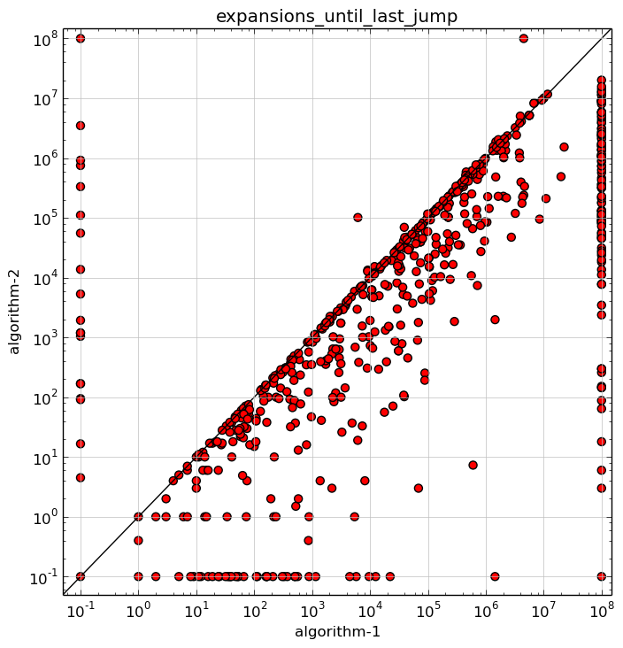
>>> exp.add_report(
...     ScatterPlotReport(
...         attributes=["expansions_until_last_jump"],
...         filter_algorithm=["algorithm-1", "algorithm-2"],
...         get_category=domain_as_category,
...         format="png",  # Use "tex" for pgfplots output.
...     ),
...     name="scatterplot-expansions",
... )
The inherited format parameter can be set to ‘png’ (default), ‘eps’, ‘pdf’, ‘pgf’ (needs matplotlib 1.2) or ‘tex’. For the latter a pgfplots plot is created.
If title is given it will be used for the name of the plot. Otherwise, the only given attribute will be the title. If none is given, there will be no title.
scale can have the values ‘linear’, ‘log’ or ‘symlog’. If omitted, a sensible default will be used for some standard attributes and ‘log’ otherwise. Relative scatter plots always use a logarithmic scaling for the y axis.
xlabel and ylabel are the axis labels.
matplotlib_options may be a dictionary of matplotlib rc parameters (see http://matplotlib.org/users/customizing.html):
>>> from downward.reports.scatter import ScatterPlotReport
>>> matplotlib_options = {
...     "font.family": "serif",
...     "font.weight": "normal",
...     # Used if more specific sizes not set.
...     "font.size": 20,
...     "axes.labelsize": 20,
...     "axes.titlesize": 30,
...     "legend.fontsize": 22,
...     "xtick.labelsize": 10,
...     "ytick.labelsize": 10,
...     "lines.markersize": 10,
...     "lines.markeredgewidth": 0.25,
...     "lines.linewidth": 1,
...     # Width and height in inches.
...     "figure.figsize": [8, 8],
...     "savefig.dpi": 100,
... }
>>> report = ScatterPlotReport(
...     attributes=["initial_h_value"], matplotlib_options=matplotlib_options
... )
You can see the full list of matplotlib options and their defaults by executing
import matplotlib
print(matplotlib.rcParamsDefault)